on
Tennis Court Detection
이번 프로젝트의 요구사항 중 하나는 촬영된 테니스 경기영상을 하늘에서 내려보는듯한 미니맵을 보여주는 것이다.
아시다시피 카메라 위치는 일반적으로 플레이어 뒷편에 있기에 위 요구사항에 만족시키려면 영상처리에서의 와핑 변환을 사용해야한다.
하지만 와핑 변환을 위해서는 영상속 테니스 코트에서 모서리의 좌표를 정확하게 알아야하는데 이 과정이 생각보다 쉽진 않다. 다음의 문제점들이 있는데
- 유저가 촬영한 영상은 항상
정면이 아닐수도 있다. - 연습경기장의
상황이 다 다르다.(코트의 색상, 화면속에 보이는 또 다른 경기장) - 카메라의
화각으로 인해 일부 모서리가 보이지 않을 수 있다. - 날씨 또는
조명문제
앞으로 포스팅 할 부분은 위 문제점을 최대한 해결하면서 테니스코트를 검출하고 나아가 와핑변환의 이해도에 초점을 맞추어 진행하겠다.
개발환경
- PC: Mac mini M1
- OS: macOS Big Sur
- Lang: Python
- Package: opencv-python, numpy
코트 검출 과정
목표는 미니맵 위에서 정확한 공의 위치이다. 이 미니맵을 만들기 위해서는 필수적으로 와핑변환을 수행하여야 하는데 현재 플레이되는 테니스코트의 모서리를 정확하게 검출해야한다.
기본적으로 색상검출이나 코너인식은 우리가 원하는 코트 검출에 도움이 크게 되지 않는다. 색상검출은 조명에 영향이 크며 연습 경기장들의 색상이 동일하지 않기 때문이다.
테니스코트가 사각형태임으로 코너 검출을 고려해볼수 있지만 화면속 다른 코트들이나 코너로 오인되는 곳들이 너무나 많다. 위 환경에서 변하지 않는 것을 굳이 찾아보자면 테니스 코트의 라인이다.
테니스 코트 라인은 실제 경기를 하는 사람의 입장에서도 필요한 요소이기에 어떤한 영상이라도 라인은 그려져있다.
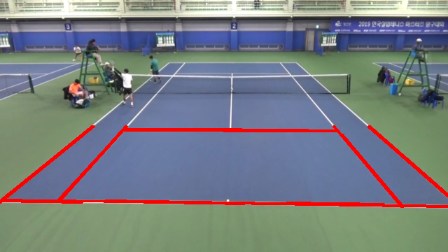
이 라인검출을 시작으로
- 검출된 라인
필터링 수직,수평선분의접점계산레퍼런스테니스 코트와의템플릿매칭으로 메인 테니스코트를 찾는 과정으로 진행해볼 것이다.
와핑 변환에 대해서
코트 검출에 전에 와핑 변환에 대한 이해도가 필요하다. 와핑을 간단히 설명하자면 좌표변환을 하기 위한 매트릭스를 구하는거라 생각하면 쉽다.
아래의 예시를 한번 보자
1차원 X선상에서
x1(0), x2(10) 점을 가진 A라인과
x1'(50) x2'(100) 점을 가진 B라인이 잇을때
각 x1 === x1', x2 === x2' 매핑되는 존재이면 A라인에서의 x3(3)은 B라인에서 얼마의 값일까?
위 예시는 간단히 0 x M = 50, 10 x M = 100 이 되는 M을 연립으로 찾으면 된다. 대략 M을 구한 뒤 3 * M하면 65라는것을 알수있다.
 테니스코트도 마찬가지이다. 실제 영상속의 테니스코트의 점 4개가 미니맵상 해당하는 위치와 매핑한 후
 기하학적 변환할 수 있는 매트릭스를 연립하여 구해주면 된다. 4개의 포인트에서 2차원으로 변환되어야 하기에 매트릭스가 다소 복잡하지만 다행히 opencv 에서는 계산하는 라이브러리를 제공하고있다.
import numpy as np
def calculate_matrix(src_points, dst_points):
    """
    Example:
        >>> scr_points = ((x1, y1), (x2, y2), (x2, y3), (x4, y4))
        >>> dst_points = ((x1', y1'), (x2', y2'), (x2', y3'), (x4', y4'))
        >>> matrix = calculate_matrix(src_points, dst_point)
    """
    src_points = np.array(src_points, dtype=np.float32)
    dst_points = np.array(dst_points, dtype=np.float32)
    return cv.getPerspectiveTransform(src_points, dst_points)
matrix가 구해지면 포인트 변환은 아주 쉽다.
def get_trans(x, y):
    point = np.array([[[x, y]]], dtype=np.float32)
    trans = cv.perspectiveTransform(point, matrix)
    return trans.reshape(-1,)
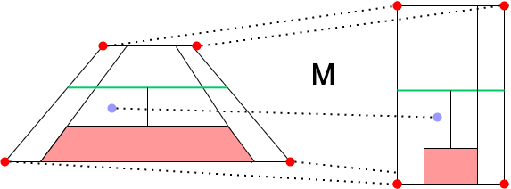
 여기서 중요한 점은 와핑 매트릭스의
 특성상 테니스 코트 내부의 어떤 위치를 기준으로 정하더라도 상관 없다는 것이다. 테니스코트 전체를 미니맵상 전체를 매핑하는 것과 코트 일부분을 미니맵상 일부분과 매핑하는 그 매트릭스는 동일하기 때문이다.
이 부분은 우리가 코트 검출에 있어 각도상 보이지 않는 테니스 코트 모서리를 찾을 필요가 없어진다.
화면상 테니스 내부에 있는 일부분만을 잡아내더라도 같은 효과를 볼 수 있다.
Preprocessing
코트 검출 과정에서 설명하였듯이 전처리는 코트의 라인을 검출하는 것에 집중하고자한다.
우선 화면에 등장하는 모든 라인을 255 나머지는 0으로 만들어보자
import cv2 as cv
class TennisCourtDetection:
    ...
    def get_binary_image(self, frame):
        gray = cv.cvtColor(image, cv.COLOR_BGR2GRAY)
        gray = cv.GaussianBlur(gray, (7, 7), 0)
        binary = cv.adaptiveThreshold(gray, 255,
                cv.ADAPTIVE_THRESH_GAUSSIAN_C,
                cv.THRESH_BINARY, 7, -1)
        return binary
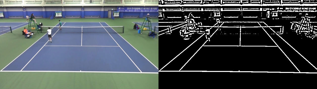 gray 영상으로 변환하고
 adaptiveThreshold을 이용했다. 물론 Edge검출도 괜찮은 방법이지만 최대한 라인을 많이 그려내야하기에 지역적 이진화 방법을 수행하였다.
우리가 사용할 라인검출은 Hough Transform를 사용할 것이다. 해당 함수를 실행하면 무수히 많은 라인들이 검출된다. 불필요한 부분들을 조금이나 제거해주기 위해 영상의 절반을 제거하자.
import cv2 as cv
class TennisCourtDetection:
    ...
    def get_remove_area(self, frame):
        binary = self.get_binary_image(image)
        binary[0:int(binary.shape[0]/2),:] = 0
        return binary
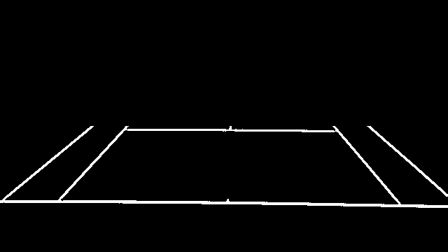
우리의 프로세스는 영상의 테니스 코트 하단에 집중하기 때문에 상단 절반을 제거해주었다.
현재의 과정에서 라인검출을 수행해주자
import numpy as np
class TennisCourtDetection:
    ...
    def __hough_transform(self, image):
        """
        Determine and cut the region of interest in the input image.
            Parameters:
                image: The output of a Canny transform.
        """
        rho = 1              #Distance resolution of the accumulator in pixels.
        theta = np.pi/180    #Angle resolution of the accumulator in radians.
        threshold = 60       #Only lines that are greater than threshold will be returned.
        minLineLength = 100   #Line segments shorter than that are rejected.
        maxLineGap = 10    #Maximum allowed gap between points on the same line to link them
        lines = cv.HoughLinesP(image, rho = rho, theta = theta, threshold = threshold,
                            minLineLength = minLineLength, maxLineGap = maxLineGap)
        if lines is None: return []
        return lines

    def get_hough_line(self, frame):
        binary = self.get_remove_area(frame)
        lines = self.__hough_transform(binary)
        lines = np.squeeze(lines) # 불필요한 차원 1개 추가 되기에 제거해준다.
        return lines
Hough Transform에 관련된 자료는 구글에 아주 많이 나와있으니 참고바란다.
한번 라인을 화면으로 출력해보자
detect = TennisCourtDetection()
def test_line(frame):
    lines = detect.get_hough_line(frame)
    for line in lines:
        x1, y1, x2, y2 = line
        cv.line(frame, (int(x1), int(y1)), (int(x2), int(y2)), color, thickness)
    return frame
라인 필터
위 그림에서는 나타나진 않았지만 라인이 겹쳐져 그려져있다.
다음 요구사항의 라인 필터링이 필요하다.
- 라인을
수직,수평으로 구분이 필요 - 비슷한 방향성을 가진 라인은 1개로
Merge
라인 필터를 수행하기 전에 필요한 수학적인 기하함수들을 구현해보자
# geomath.py
def is_horizon(self, line):
    x1, y1, x2, y2 = line
    dx = abs(x1 - x2)
    dy = abs(y1 - y2)
    return dx > 4 * dy

def get_contact_4point(x11, y11, x12, y12, x21, y21, x22, y22):
    if x12 == x11 or x22 == x21:
        if x12 == x11:
            cx = x12
            m2 = (y22 - y21) / (x22 - x21)
            cy = m2 * (cx - x21) + y21
            return cx, cy
        if x22 == x21:
            cx = x22
            m1 = (y12 - y11) / (x12 - x11)
            cy = m1 * (cx - x11) + y11
            return cx, cy

    m1 = (y12 - y11) / (x12 - x11)
    m2 = (y22 - y21) / (x22 - x21)
    if m1 == m2:
        print('parallel')
        return None
    cx = (x11 * m1 - y11 - x21 * m2 + y21) / (m1 - m2)
    cy = m1 * (cx - x11) + y11

    return cx, cy

def get_contact_2line(line1, line2):
    x11, y11, x12, y12 = line1
    x21, y21, x22, y22 = line2
    return get_contact_4point(x11, y11, x12, y12, x21, y21, x22, y22)
이제 위 기하함수를 이용하여 라인을 수직, 수평으로 분리해보자
from .geomath import *
class TennisCourtDetection:
    ...
    def __separate(self, lines):
        """
        Separate line to vertical and horizontal lines
            Parameter:
                lines: cv.houghLineP()
            Return:
                horizontal, vertical
        """
        horizontal = []
        vertical = []
        for line in lines:
            if is_horizon(line):
                horizontal.append(line)
            else:
                vertical.append(line)

        return horizontal, vertical

    def get_court_line(self, frame):
        lines = self.get_hough_line(frame)
    #    lines = [ Line(line) for line in lines ]
        hori, vert = self.__separate(lines)
        return hori, vert
is_horizon()를 보면 각 라인의 기울기의 Threshold에 따라 결정된다.
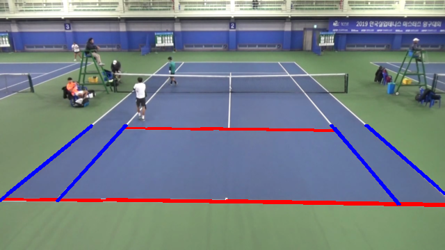
분리된 두 라인들을 각각 그려보면
detect = TennisCourtDetection()
def test_line(frame):
    hori, cert = detect.get_court_line(frame)
    for line in hori:
        x1, y1, x2, y2 = line
        cv.line(frame, (int(x1), int(y1)), (int(x2), int(y2)), color=[0, 0, 255], thickness=2)
    for line in vert:
        x1, y1, x2, y2 = line
        cv.line(frame, (int(x1), int(y1)), (int(x2), int(y2)), color=[255, 0, 0], thickness=2)
    return frame
라인 접점
코트에서 추출된 수직,수평 선분들을 구해서 모든 경우의 quadrangle을 찾는다. x, y 우선순위를 가지는 sorting도 수행해주자
from .geomath import get_contact_2line
class TennisCorutDetection:
    ...
    def _sort_interaction(self, points):
        sorted_y = sorted(points, key=lambda x: x[1])
        p12 = sorted_y[:2]
        p34 = sorted_y[2:]
        p12 = sorted(p12, key=lambda x: x[0])
        p34 = sorted(p34, key=lambda x: x[0])
        return p12 + p34

    def get_quadrangles(self, frame):
            hori, vert = self.get_court_line(frame)
            quadrangles = []
            for h1, h2 in list(combinations(hori, 2)):
                for v1, v2 in list(combinations(vert, 2)):
                    p1 = get_contact_2line(h1, v1)
                    p2 = get_contact_2line(h1, v2)
                    p3 = get_contact_2line(h2, v1)
                    p4 = get_contact_2line(h2, v2)

                    points = [p1, p2, p3, p4]
                    points = self._sort_interaction(points)
                    quadrangles.append(points)

        return quadrangles
Template matching
Template matching은 원본 이미지에서 Templete 이미지와 가장 비슷한 영역을 찾는 이미지 처리기술이다.
테니스 코트에서는 원본영상의 코트와 실제 규약을 따르는 레퍼런스 코트를 비교할 것이다.
테니스 코트 검출의 Flow를 다시 한번 설명하자면
- 라인검출을 통해 영상에서
모든 라인들을 찾는다. - 라인들을 수평, 수직으로
분류 - 임의의 수평 2개, 수직 2개의 라인에서 각 라인이 만나는
접점을 구한다. - 4-Point를 와핑하여 레퍼런스와
Template maching을 시도 Score가 가장 좋은 4-Point를 선택
이고 여기서 우리는 레퍼런스 코트를 구현하는 방법과 그것을 실제 원본영상에서 어떻게 비교하는지에 대해 중점적으로
포스팅 할 것이다.
Court Reference
영상에 촬영된 코트는 실제로 정해진 규격이 있다. 이 규격에 맞는 레퍼런스 코트를 코드화해보자
#reference.py
class CourtReference:
    def __init__(self, path):
        self._path = path
        self.__init()
        self.__construct()

    def __init(self):
        self._image = cv.imread(self._path)
        self._height, self._width = self._image.shape[:2]

    def __construct(self):
        self.basetopline = ((286, 561), (1379, 561))
        self.basebottomline = ((286, 2935), (1379, 2935))
        self.baseleftline = ((286, 561), (286, 2935))
        self.baserightline = ((1379, 561), (1379, 2935))
        self.net = ((286, 1748), (1379, 1748))
        self.topinnerline = ((423, 1110), (1242, 1110))
        self.middleline = ((832, 1110), (832, 2386))
        self.bottominnerline = ((423, 2386), (1242, 2386))
        self.leftinnerline = ((423, 561), (423, 2935))
        self.rightinnerline = ((1242, 561), (1242, 2935))
CourtReference는 생성시에 실제 테니스 코트 규격에 맞춘 이미지의 path를 입력받고 이미지를 생성한다.
여기서 __construct는 해당 이미지의 비교할 코트의 중요 위치를 포인트화 하였다.
템플릿 매칭을 하기위해 다양한 패턴의 4포인트를 만들자. 그림을 포인트로 표현하여 구현하였다.
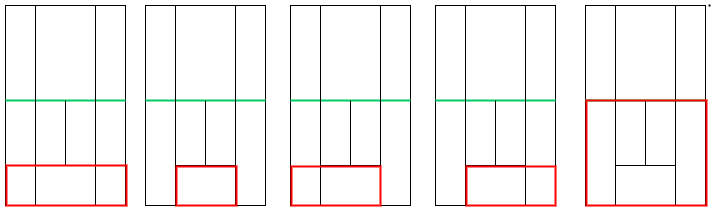
class CourtReference:
    ...
    def get_court_pattern(self):
        return {
            0: ((832, 2386), (1379, 2386), (832, 2935), (1379, 2935)),
            1: ((286, 2386), (832, 2386), (832, 2935), (286, 2935)),
            2: ((286, 2386), (1379, 2386), (832, 2935), (1379, 2935)),
            3: ((423, 2386), (1242, 2386), (423, 2935), (1242, 2935)),
            4: ((286, 1748), (1379, 1748), (286, 2935), (1379, 2935)),
        }
이제 레퍼런스 코트의 표현하는 클래스 개발을 완료했다. TennisCourtDetection 클래스로 돌아와서
스코어를 계산하는 함수를 구현해보자.
Matching Score
위 패턴과 실제 영상에서의 접점들의 매칭 스코어를 구해야한다.
class TennisCourtDetection:
    ...
    def _get_score(self, src, matching):
        capture = src.copy()
        court = matching.copy()
        capture[capture > 0] = 1
        court[court > 0] = 1
        correct = capture * court
        wrong = court - correct
        return np.sum(correct) - 0.5 * np.sum(wrong)
스코어는 높을수록 가장 비슷하다 판단할 수 있도록
두 개의 Binary 영상을 0외의 요소는 1로 두고 아래 공식으로 스코어를 계산한다.
영상의 중요한 정보에 대해서
여기서 중요하게 짚고 넘어가야할 부분이 있다. 와핑 후 두 영상을 비교하는건 맞지만
2가지 방법이 존재한다.
원본영상에서코트영상으로 와핑 후레퍼런스 코트와 비교코트영상에서원본영상으로 와핑 후원본영상과 비교
둘중 어떤 방법이 더 나은 방법으로 보이는가?
필자는 처음에 1번 방식으로 진행했지만 생각보다 코트검출이 잘 되지 않았다. 반대로 2번 방법을 시도하였을땐 매우 높은 확률로 검출 되었다. 어떠한 차이가 있었던 것 일까?
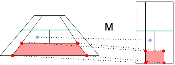
아래 그림을 보자
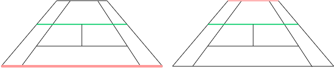
기울진 테니스 코트에서 두 그림의 라인중에 어떤 부분이 더 중요한지 고민해보자
정답은 왼쪽 그림에 있는 라인이 더 중요하다. 이유는 영상에서 보면 오른쪽 그림의 라인은 잘 보이지도 않을뿐더러 실제로 사람이 보아도 왼쪽라인에 더 집중이 되기 때문이다.
이처럼 영상에서 상대적으로 중요한 정보량을 표시해주는 부분이 존재한다.
위 2가지 방법중 1번 방식의 경우 크게 중요하지 않는 부분이 강조되어 매칭되는 반면
2번의 경우는 실제 코트가 더 중요한 부분을 부각시켜주는 효과가 있기에 2번 방식을 채택해야한다.
기존 Image ➞ Court 로 변환하는 Matrix를 Court ➞ Image 로 변환시키는 Inverse Matrix를 구해보자
코드는 간단하다.
def inverse(matrix):
    return cv.invert(matrix)[1]
이제 라인 점접에서 모든 접점과 패턴을 비교하는 bruteforce를 진행하자.
class TennisCorutDetection:
    ...
    def bruteforce(self, quadrangles):
        max_score = 0
        max_matrix = None
        patterns = self._court_reference.get_court_pattern()
        for points in quadrangles:
            for _, pattern in patterns.items():
                matrix = cv.getPerspectiveTransform(pattern, points) # court -> game
                court_to_game = cv.warpPerspective(self._court, matrix, self._frame.shape[:2])
                score = self._get_score(self.frame, court_to_game)
                if max_score < score:
                    max_score = score
                    max_matrix = matrix

        return cv.invert(max_matrix)[1]
pattern와quadrangle를 사용하여matrix를 계산한다.- 주어진 matrix로 코트이미지를 frame크기로
와핑변환해서생성한다. - 두 영상의 스코어에서 가장 큰 스코어의
matrix로 업데이트한다.
해당 matrix는 실제 게임좌표를 코트에 매칭이 될수 있도록 변환해주는 matrix이다.
이것만 가지고있다면 실제 게임에서 발생하는 상황을 코트 위에 그대로 그려줄 수 있다.
전체 코드
import cv2 as cv
import numpy as np
from itertools import combinations
from .geomath import *
from .dataclasses import *
from .geomath import *
class TennisCourtDetection:
    def __init__(self, court_reference):
        self._court = court_reference
        self._frame = None

    def __hough_transform(self, image):
        """
        Determine and cut the region of interest in the input image.
            Parameters:
                image: The output of a Canny transform.
        """
        rho = 1              #Distance resolution of the accumulator in pixels.
        theta = np.pi/180    #Angle resolution of the accumulator in radians.
        threshold = 60       #Only lines that are greater than threshold will be returned.
        minLineLength = 100   #Line segments shorter than that are rejected.
        maxLineGap = 10    #Maximum allowed gap between points on the same line to link them
        lines = cv.HoughLinesP(image, rho = rho, theta = theta, threshold = threshold,
                            minLineLength = minLineLength, maxLineGap = maxLineGap)
        if lines is None: return []
        return lines

    def __separate(self, lines):
        """
        Separate line to vertical and horizontal lines
            Parameter:
                lines: cv.houghLineP()
            Return:
                horizontal, vertical
        """
        hori = []
        vert = []
        for line in lines:
            if is_horizon(line):
                hori.append(line)
            else:
                vert.append(line)

        return hori, vert

    def _sort_interaction(self, points):
        sorted_y = sorted(points, key=lambda x: x[1])
        p12 = sorted_y[:2]
        p34 = sorted_y[2:]
        p12 = sorted(p12, key=lambda x: x[0])
        p34 = sorted(p34, key=lambda x: x[0])
        return p12 + p34

    def _get_score(self, src, matching):
        capture = src.copy()
        court = matching.copy()
        capture[capture > 0] = 1
        court[court > 0] = 1
        correct = capture * court
        wrong = court - correct
        return np.sum(correct) - 0.5 * np.sum(wrong)

    def get_binary_image(self, frame):
        gray = cv.cvtColor(frame, cv.COLOR_BGR2GRAY)
        gray = cv.GaussianBlur(gray, (7, 7), 0)
        binary = cv.adaptiveThreshold(gray, 255,
                cv.ADAPTIVE_THRESH_GAUSSIAN_C,
                cv.THRESH_BINARY, 7, -1)
        return binary

    def get_remove_area(self, image):
        binary = self.get_binary_image(image)
        binary[0:int(binary.shape[0]/2),:] = 0
        return binary

    def get_hough_line(self, frame):
        binary = self.get_remove_area(frame)
        lines = self.__hough_transform(binary)
        lines = np.squeeze(lines)
        return lines

    def get_court_line(self, frame):
        lines = self.get_hough_line(frame)
        hori, vert = self.__separate(lines)
        return hori, vert

    def get_quadrangles(self, frame):
        hori, vert = self.get_court_line(frame)
        quadrangles = []
        for h1, h2 in list(combinations(hori, 2)):
            for v1, v2 in list(combinations(vert, 2)):
                p1 = get_contact_2line(h1, v1)
                p2 = get_contact_2line(h1, v2)
                p3 = get_contact_2line(h2, v1)
                p4 = get_contact_2line(h2, v2)

                points = [p1, p2, p3, p4]
                points = self._sort_interaction(points)
                quadrangles.append(points)

        return quadrangles

    def bruteforce(self, quadrangles):
        max_score = 0
        max_matrix = None
        patterns = self._court_reference.get_court_pattern()
        for points in quadrangles:
            for _, pattern in patterns.items():
                matrix = cv.getPerspectiveTransform(pattern, points) # court -> game
                court_to_game = cv.warpPerspective(self._court, matrix, self._frame.shape[:2])
                score = self._get_score(self.frame, court_to_game)
                if max_score < score:
                    max_score = score
                    max_matrix = matrix

        return cv.invert(max_matrix)[1]

    def detect(self, frame):
        self._frame = frame
        quadrangles = self.get_quadrangles(frame)
        return self.bruteforce(quadrangles)
…
코드를 자세히보면 상당히 연산량이 많다. 실제로 돌려보면 매 프레임마다 딜레이가 많이 발생하여 실시간으로 코트검출 하는 것에는 다소 무리가 있다. 그래서 영상 초반부에 1~2개 정도의 프레임만 검출하여 나머지 영상에는 고정값으로 가져가는 방식으로 진행하길 추천한다.
다음은 추가해볼 수 있는 사항이다.
- 라인 검출 이후 라인 트레이싱
- bruteforce 방식에 memory를 추가하여 memoization으로 변경
- 딥러닝 도입
앞서 배운 것들을 파이썬에서 쉽게 배포가능하도록 패키징 작업을 하고 실제 영상을 불러와 인코딩하는 과정을 다음 포스팅에서 진행할 것이다.